maartengrootendorst.com - A Visual Guide to Quantization

Demystifying the Compression of Large Language Models

Translations - Korean - Chinese - French

As their name suggests, Large Language Models (LLMs) are often too large to run on consumer hardware. These models may exceed billions of parameters and generally need GPUs with large amounts of VRAM to speed up inference.

As such, more and more research has been focused on making these models smaller through improved training, adapters, etc. One major technique in this field is called quantization.

In this post, I will introduce the field of quantization in the context of language modeling and explore concepts one by one to develop an intuition about the field. We will explore various methodologies, use cases, and the principles behind quantization.

In this visual guide, there are more than 50 custom visuals to help you develop an intuition about quantization!

To see more visualizations related to LLMs and to support this newsletter, check out the book I wrote on Large Language Models!

Official website of the book. You can order the book on Amazon. All code is uploaded to GitHub.

P.S. If you read the book, a quick review would mean the world—it really helps us authors!

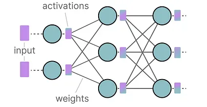
Part 1: The “Problem“ with LLMs

LLMs get their name due to the number of parameters they contain. Nowadays, these models typically have billions of parameters (mostly weights) which can be quite expensive to store.

During inference, activations are created as a product of the input and the weights, which similarly can be quite large.

As a result, we would like to represent billions of values as efficiently as possible, minimizing the amount of space we need to store a given value.

Let’s start from the beginning and explore how numerical values are represented in the first place before optimizing them.

How to Represent Numerical Values

A given value is often represented as a floating point number (or floats in computer science): a positive or negative number with a decimal point.

These values are represented by “ bits ”, or binary digits. The IEEE-754 standard describes how bits can represent one of three functions to represent the value: the sign, exponent, or fraction (or mantissa).

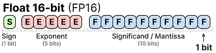
Together, these three aspects can be used to calculate a value given a certain set of bit values:

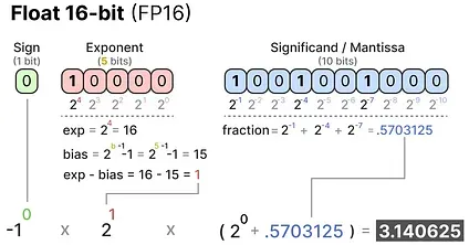
The more bits we use to represent a value, the more precise it generally is:

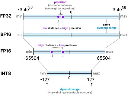
Memory Constraints

The more bits we have available, the larger the range of values that can be represented.

The interval of representable numbers a given representation can take is called the dynamic range whereas the distance between two neighboring values is called precision.

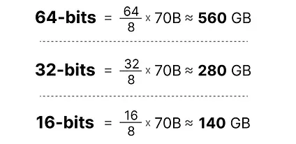
A nifty feature of these bits is that we can calculate how much memory your device needs to store a given value. Since there are 8 bits in a byte of memory, we can create a basic formula for most forms of floating point representation.

NOTE: In practice, more things relate to the amount of (V)RAM you need during inference, like the context size and architecture.

Now let’s assume that we have a model with 70 billion parameters. Most models are natively represented with float 32-bit (often called full-precision), which would require 280GB of memory just to load the model.

As such, it is very compelling to minimize the number of bits to represent the parameters of your model (as well as during training!). However, as the precision decreases the accuracy of the models generally does as well.

We want to reduce the number of bits representing values while maintaining accuracy… This is where quantization comes in!

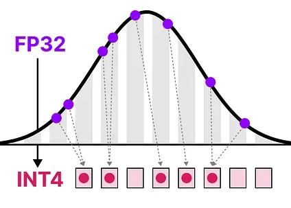
Part 2: Introduction to Quantization

Quantization aims to reduce the precision of a model’s parameter from higher bit-widths (like 32-bit floating point) to lower bit-widths (like 8-bit integers).

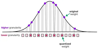
There is often some loss of precision (granularity) when reducing the number of bits to represent the original parameters.

To illustrate this effect, we can take any image and use only 8 colors to represent it:

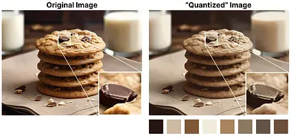
Image adapted from the original by Slava Sidorov.

Notice how the zoomed-in part seems more “grainy” than the original since we can use fewer colors to represent it.

The main goal of quantization is to reduce the number of bits (colors) needed to represent the original parameters while preserving the precision of the original parameters as best as possible.

Common Data Types

First, let’s look at common data types and the impact of using them rather than 32-bit (called full-precision or FP32) representations.

FP16

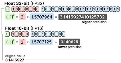
Let’s look at an example of going from 32-bit to 16-bit (called half precision or FP16) floating point:

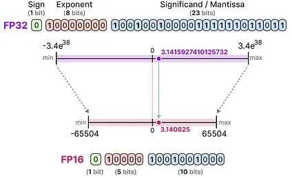
Notice how the range of values FP16 can take is quite a bit smaller than FP32.

BF16

To get a similar range of values as the original FP32, bfloat 16 was introduced as a type of “truncated FP32”:

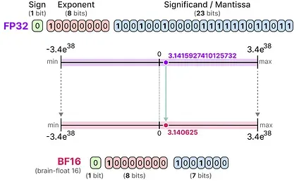
BF16 uses the same amount of bits as FP16 but can take a wider range of values and is often used in deep learning applications.

INT8

When we reduce the number of bits even further, we approach the realm of integer-based representations rather than floating-point representations. To illustrate, going FP32 to INT8, which has only 8 bits, results in a fourth of the original number of bits:

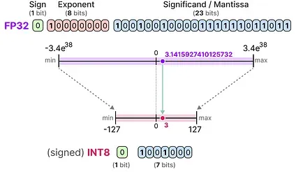
Depending on the hardware, integer-based calculations might be faster than floating-point calculations but this isn’t always the case. However, computations are generally faster when using fewer bits.

For each reduction in bits, a mapping is performed to “squeeze” the initial FP32 representations into lower bits.

In practice, we do not need to map the entire FP32 range [-3.4e38, 3.4e38] into INT8. We merely need to find a way to map the range of our data (the model’s parameters) into INT8.

Common squeezing/mapping methods are symmetric and asymmetric quantization and are forms of linear mapping.

Let’s explore these methods to quantize from FP32 to INT8.

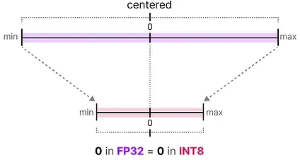
Symmetric Quantization

In symmetric quantization, the range of the original floating-point values is mapped to a symmetric range around zero in the quantized space. In the previous examples, notice how the ranges before and after quantization remain centered around zero.

This means that the quantized value for zero in the floating-point space is exactly zero in the quantized space.

A nice example of a form of symmetric quantization is called absolute maximum (absmax) quantization.

Given a list of values, we take the highest absolute value (α) as the range to perform the linear mapping.

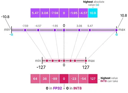
Note the [-127, 127] range of values represents the restricted range. The unrestricted range is [-128, 127] and depends on the quantization method.

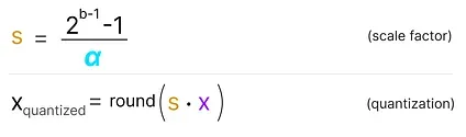
Since it is a linear mapping centered around zero, the formula is straightforward.

We first calculate a scale factor (s) using:

• b is the number of bytes that we want to quantize to (8),
• α is the highest absolute value,

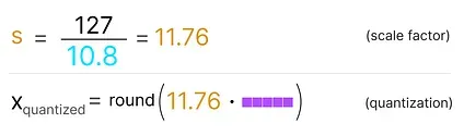
Then, we use the s to quantize the input x:

Filling in the values would then give us the following:

To retrieve the original FP32 values, we can use the previously calculated scaling factor (s) to dequantize the quantized values.

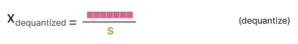
Applying the quantization and then dequantization process to retrieve the original looks as follows:

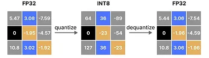
You can see certain values, such as 3.08 and 3.02 being assigned to the INT8, namely 36. When you dequantize the values to return to FP32, they lose some precision and are not distinguishable anymore.

This is often referred to as the quantization error which we can calculate by finding the difference between the original and dequantized values.

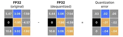
Generally, the lower the number of bits, the more quantization error we tend to have.

Asymmetric Quantization

Asymmetric quantization, in contrast, is not symmetric around zero. Instead, it maps the minimum (β) and maximum (α) values from the float range to the minimum and maximum values of the quantized range.

The method we are going to explore is called zero-point quantization.

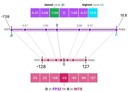
Notice how the 0 has shifted positions? That’s why it’s called asymmetric quantization. The min/max values have different distances to 0 in the range [-7.59, 10.8].

Due to its shifted position, we have to calculate the zero-point for the INT8 range to perform the linear mapping. As before, we also have to calculate a scale factor (s) but use the difference of INT8’s range instead [-128, 127]

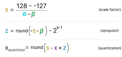
Notice how this is a bit more involved due to the need to calculate the zeropoint (z) in the INT8 range to shift the weights.

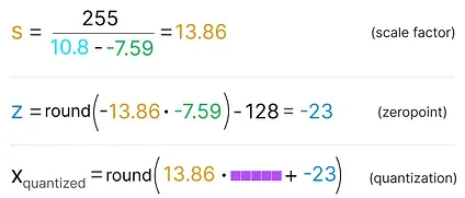
As before, let’s fill in the formula:

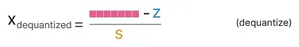
To dequantize the quantized from INT8 back to FP32, we will need to use the previously calculated scale factor (s) and zeropoint (z).

Other than that, dequantization is straightforward:

When we put symmetric and asymmetric quantization side-by-side, we can quickly see the difference between methods:

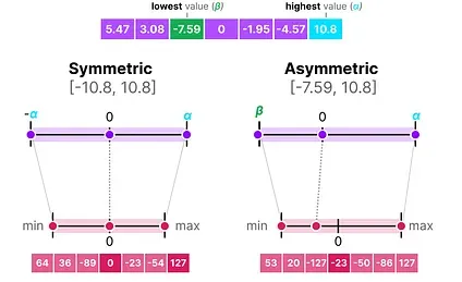
Note the zero-centered nature of symmetric quantization versus the offset of asymmetric quantization.

Range Mapping and Clipping

In our previous examples, we explored how the range of values in a given vector could be mapped to a lower-bit representation. Although this allows for the full range of vector values to be mapped, it comes with a major downside, namely outliers.

Imagine that you have a vector with the following values:

Note how one value is much larger than all others and could be considered an outlier. If we were to map the full range of this vector, all small values would get mapped to the same lower-bit representation and lose their differentiating factor:

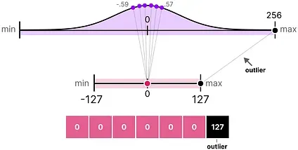
This is the absmax method we used earlier. Note that the same behavior happens with asymmetric quantization if we do not apply clipping.

Instead, we can choose to clip certain values. Clipping involves setting a different dynamic range of the original values such that all outliers get the same value.

In the example below, if we were to manually set the dynamic range to [-5, 5] all values outside that will either be mapped to -127 or to 127 regardless of their value:

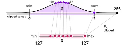
The major advantage is that the quantization error of the non-outliers is reduced significantly. However, the quantization error of outliers increases.

Calibration

In the example, I showed a naive method of choosing an arbitrary range of [-5, 5]. The process of selecting this range is known as calibration which aims to find a range that includes as many values as possible while minimizing the quantization error.

Performing this calibration step is not equal for all types of parameters.

Weights (and Biases)

We can view the weights and biases of an LLM as static values since they are known before running the model. For instance, the ~20GB file of Llama 3 consists mostly of its weight and biases.

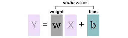
Since there are significantly fewer biases (millions) than weights (billions), the biases are often kept in higher precision (such as INT16), and the main effort of quantization is put towards the weights.

For weights, which are static and known, calibration techniques for choosing the range include:

• Manually chosing a percentile of the input range
• Optimize the mean squared error (MSE) between the original and quantized weights.
• Minimizing entropy (KL-divergence) between the original and quantized values

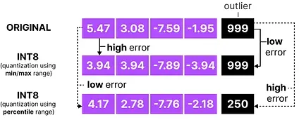
Choosing a percentile, for instance, would lead to similar clipping behavior as we have seen before.

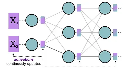
Activations

The input that is continuously updated throughout the LLM is typically referred to as “ activations ”.

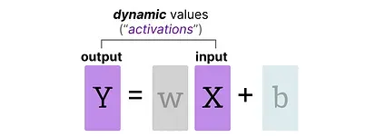
Note that these values are called activations since they often go through some activation function, like sigmoid or relu.

Unlike weights, activations vary with each input data fed into the model during inference, making it challenging to quantize them accurately.

Since these values are updated after each hidden layer, we only know what they will be during inference as the input data passes through the model.

Broadly, there are two methods for calibrating the quantization method of the weights and activations:

• Post-Training Quantization (PTQ)
  • Quantization after training
• Quantization Aware Training (QAT)
  • Quantization during training/fine-tuning

Part 3: Post-Training Quantization

One of the most popular quantization techniques is post-training quantization (PTQ). It involves quantizing a model’s parameters (both weights and activations) after training the model.

Quantization of the weights is performed using either symmetric or asymmetric quantization.

Quantization of the activations, however, requires inference of the model to get their potential distribution since we do not know their range.

There are two forms of quantization of the activations:

• Dynamic Quantization
• Static Quantization

Dynamic Quantization

After data passes a hidden layer, its activations are collected:

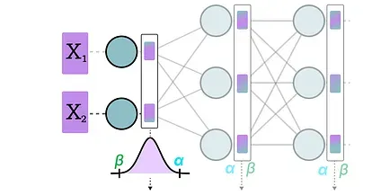
This distribution of activations is then used to calculate the zeropoint (z) and scale factor (s) values needed to quantize the output:

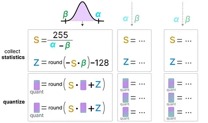
The process is repeated each time data passes through a new layer. Therefore, each layer has its own separate z and s values and therefore different quantization schemes.

Static Quantization

In contrast to dynamic quantization, static quantization does not calculate the zeropoint (z) and scale factor (s) during inference but beforehand.

To find those values, a calibration dataset is used and given to the model to collect these potential distributions.

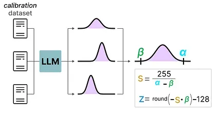
After these values have been collected, we can calculate the necessary s and z values to perform quantization during inference.

When you are performing actual inference, the s and z values are not recalculated but are used globally over all activations to quantize them.

In general, dynamic quantization tends to be a bit more accurate since it only attempts to calculate the s and z values per hidden layer. However, it might increase compute time as these values need to be calculated.

In contrast, static quantization is less accurate but is faster as it already knows the s and z values used for quantization.

The Realm of 4-bit Quantization

Going below 8-bit quantization has proved to be a difficult task as the quantization error increases with each loss of bit. Fortunately, there are several smart ways to reduce the bits to 6, 4, and even 2-bits (although going lower than 4-bits using these methods is typically not advised).

We will explore two methods that are commonly shared on HuggingFace:

• GPTQ (full model on GPU)
• GGUF (potentially offload layers on the CPU)

GPTQ

GPTQ is arguably one of the most well-known methods used in practice for quantization to 4-bits.¹

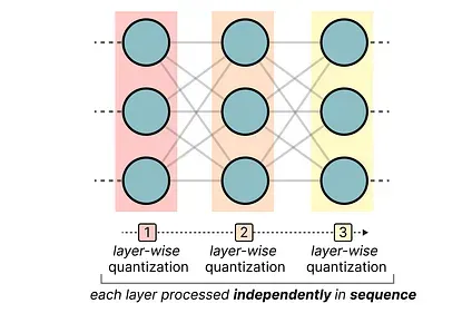
It uses asymmetric quantization and does so layer by layer such that each layer is processed independently before continuing to the next:

During this layer-wise quantization process, it first converts the layer’s weights into the inverse- Hessian. It is a second-order derivative of the model’s loss function and tells us how sensitive the model’s output is to changes in each weight.

Simplified, it essentially demonstrates the (inverse) importance of each weight in a layer.

Weights associated with smaller values in the Hessian matrix are more crucial because small changes in these weights can lead to significant changes in the model’s performance.

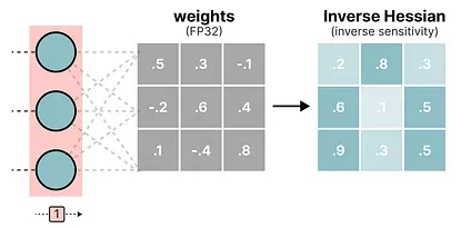
In the inverse-Hessian, lower values indicate more “important” weights.

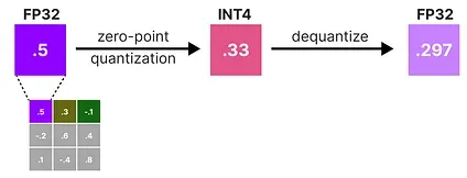
Next, we quantize and then dequantize the weight of the first row in our weight matrix:

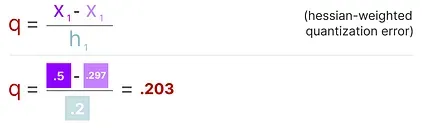
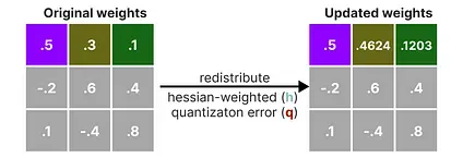
This process allows us to calculate the quantization error (q) which we can weigh using the inverse-Hessian (h_1) that we calculated beforehand.

Essentially, we are creating a weighted-quantization error based on the importance of the weight:

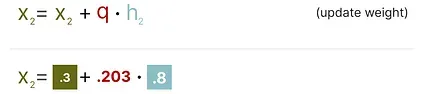
Next, we redistribute this weighted quantization error over the other weights in the row. This allows for maintaining the overall function and output of the network.

For example, if we were to do this for the second weight, namely.3 (x_2), we would add the quantization error (q) multiplied by the inverse-Hessian of the second weight (h _2)

We can do the same process over the third weight in the given row:

We iterate over this process of redistributing the weighted quantization error until all values are quantized.

This works so well because weights are typically related to one another. So when one weight has a quantization error, related weights are updated accordingly (through the inverse-Hessian).

NOTE: The authors used several tricks to speed up computation and improve performance, such as adding a dampening factor to the Hessian, “lazy batching”, and precomputing information using the Cholesky method. I would highly advise checking out this YouTube video on the subject.

TIP: Check out EXL2 if you want a quantization method aimed at performance optimizations and improving inference speed.

GGUF

While GPTQ is a great quantization method to run your full LLM on a GPU, you might not always have that capacity. Instead, we can use GGUF to offload any layer of the LLM to the CPU. ²

This allows you to use both the CPU and GPU when you do not have enough VRAM.

The quantization method GGUF is updated frequently and might depend on the level of bit quantization. However, the general principle is as follows.

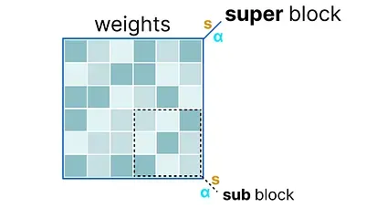
First, the weights of a given layer are split into “super” blocks each containing a set of “sub” blocks. From these blocks, we extract the scale factor (s) and alpha (α):

To quantize a given “sub” block, we can use the absmax quantization we used before. Remember that it multiplies a given weight by the scale factor (s):

The scale factor is calculated using the information from the “sub” block but is quantized using the information from the “super” block which has its own scale factor:

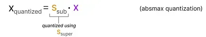
This block-wise quantization uses the scale factor (s_super) from the “super” block to quantize the scale factor (s_sub) from the “sub” block.

The quantization level of each scale factor might differ with the “super” block generally having a higher precision than the scale factor of the “sub” block.

To illustrate, let’s explore a couple of quantization levels (2-bit, 4-bit, and 6-bit):

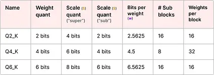
NOTE: Depending on the quantization type, an additional minimum value ( m ) is needed to adjust the zero-point. These are quantized the same as the scale factor ( s ).

Check out the original pull request for an overview of all quantization levels. Also, see this pull request for more information on quantization using importance matrices.

Part 4: Quantization Aware Training

In Part 3, we saw how we could quantize a model after training. A downside to this approach is that this quantization does not consider the actual training process.

This is where Quantization Aware Training (QAT) comes in. Instead of quantizing a model after it was trained with post-training quantization (PTQ), QAT aims to learn the quantization procedure during training.

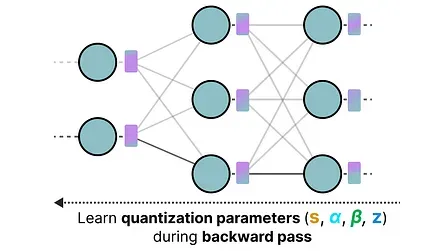
QAT tends to be more accurate than PTQ since the quantization was already considered during training. It works as follows:

During training, so-called “ fake ” quants are introduced. This is the process of first quantizing the weights to, for example, INT4 and then dequantizing back to FP32:

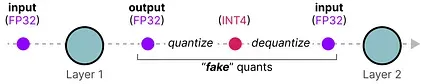
This process allows the model to consider the quantization process during training, the calculation of loss, and weight updates.

QAT attempts to explore the loss landscape for “ wide ” minima to minimize the quantization errors as “ narrow ” minima tend to result in larger quantization errors.

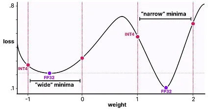
For example, imagine if we did not consider quantization during the backward pass. We choose the weight with the smallest loss according to gradient descent. However, that would introduce a larger quantization error if it’s in a “ narrow ” minima.

In contrast, if we consider quantization, a different updated weight will be selected in a “ wide ” minima with a much lower quantization error.

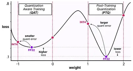
As such, although PTQ has a lower loss in high precision (e.g., FP32), QAT results in a lower loss in lower precision (e.g., INT4) which is what we aim for.

The Era of 1-bit LLMs: BitNet

Going to 4-bits as we saw before is already quite small but what if we were to reduce it even further?

This is where BitNet comes in, representing the weights of a model single 1-bit, using either -1 or 1 for a given weight.³

It does so by injecting the quantization process directly into the Transformer architecture.

Remember that the Transformer architecture is used as the foundation of most LLMs and is composed of computations that involve linear layers:

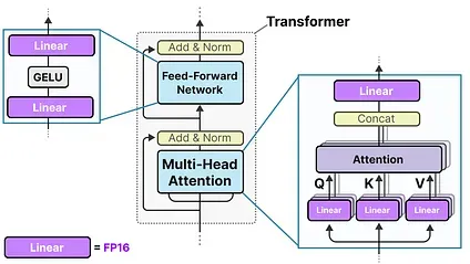
These linear layers are generally represented with higher precision, like FP16, and are where most of the weights reside.

BitNet replaces these linear layers with something they call the BitLlinear:

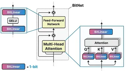
A BitLinear layer works the same as a regular linear layer and calculates the output based on the weights multiplied by the activation.

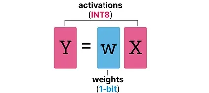
In contrast, a BitLinear layer represents the weights of a model using 1-bit and activations using INT8:

A BitLinear layer, like Quantization-Aware Training (QAT) performs a form of “fake” quantization during training to analyze the effect of quantization of the weights and activations:

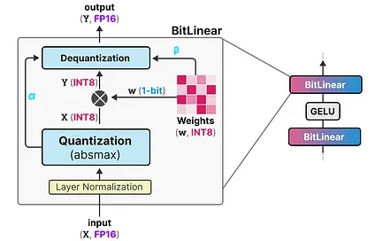
NOTE: In the paper they used γ instead of α but since we used a throughout our examples, I’m using that. Also, note that β is not the same as we used in zero-point quantization but the average absolute value.

Let’s go through the BitLinear step-by-step.

Weight Quantization

While training, the weights are stored in INT8 and then quantized to 1-bit using a basic strategy, called the signum function.

In essence, it moves the distribution of weights to be centered around 0 and then assigns everything left to 0 to be -1 and everything to the right to be 1:

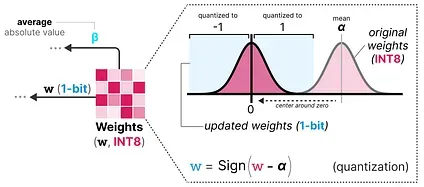
Additionally, it tracks a value β (average absolute value) that we will use later on for dequantization.

Activation Quantization

To quantize the activations, BitLinear makes use of absmax quantization to convert the activations from FP16 to INT8 as they need to be in higher precision for the matrix multiplication (×).

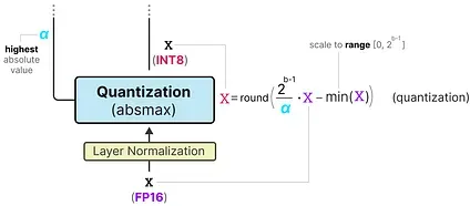
Additionally, it tracks α (highest absolute value) that we will use later on for dequantization.

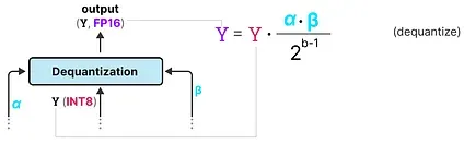
Dequantization

We tracked α (highest absolute value of activations) and β (average absolute value of weights) as those values will help us dequantize the activations back to FP16.

The output activations are rescaled with { α, γ} to dequantize them to the original precision:

And that’s it! This procedure is relatively straightforward and allows models to be represented with only two values, either -1 or 1.

Using this procedure, the authors observed that as the model size grows, the smaller the performance gap between a 1-bit and FP16-trained becomes.

However, this is only for larger models (>30B parameters) and the gab with smaller models is still quite large.

All Large Language Models are in 1.58 Bits

BitNet 1.58b was introduced to improve upon the scaling issue previously mentioned.⁴

In this new method, every single weight of the model is not just -1 or 1, but can now also take 0 as a value, making it ternary. Interestingly, adding just the 0 greatly improves upon BitNet and allows for much faster computation.

The Power of 0

So why is adding 0 such a major improvement?

It has everything to do with matrix multiplication!

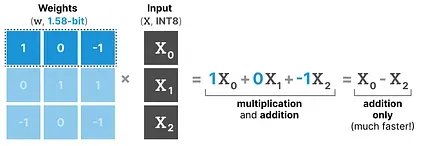
First, let’s explore how matrix multiplication in general works. When calculating the output, we multiply a weight matrix by an input vector. Below, the first multiplication of the first layer of a weight matrix is visualized:

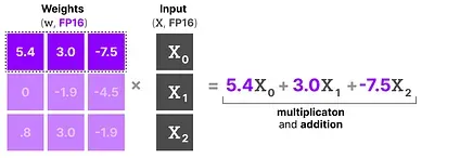
Note that this multiplication involves two actions, multiplying individual weights with the input and then adding them all together.

BitNet 1.58b, in contrast, manages to forego the act of multiplication since ternary weights essentially tell you the following:

• 1: I want to add this value
• 0: I do not want this value
• -1: I want to subtract this value

As a result, you only need to perform addition if your weights are quantized to 1.58 bit:

Not only can this speed up computation significantly, but it also allows for feature filtering.

By setting a given weight to 0 you can now ignore it instead of either adding or subtracting the weights as is the case with 1-bit representations.

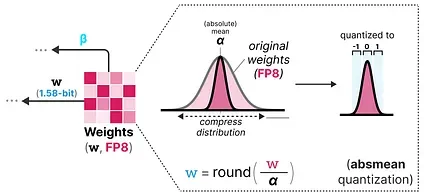
Quantization

To perform weight quantization BitNet 1.58b uses absmean quantization which is a variation of the absmax quantization that we saw before.

It simply compresses the distribution of weights and uses the absolute mean (α) to quantize values. They are then rounded to either -1, 0, or 1:

Compared to BitNet the activation quantization is the same except for one thing. Instead of scaling the activations to range [0, 2ᵇ⁻¹], they are now scaled to
[-2ᵇ⁻¹, 2ᵇ⁻¹] instead using absmax quantization.

And that’s it! 1.58-bit quantization required (mostly) two tricks:

• Adding 0 to create ternary representations [-1, 0, 1]
• absmean quantization for weights

As a result, we get lightweight models due to having only 1.58 computationally efficient bits!

Conclusion

This concludes our journey in quantization! Hopefully, this post gives you a better understanding of the potential of quantization, GPTQ, GGUF, and BitNet. Who knows how small the models will be in the future?!

To see more visualizations related to LLMs and to support this newsletter, check out the book I wrote on Large Language Models!

For more information, see the official website. Order the book on Amazon. All code will be uploaded to Github.

Resources

Hopefully, this was an accessible introduction to quantization! If you want to go deeper, I would suggest the following resources:

• A HuggingFace blog about the LLM.int8() quantization method: you can find the paper here.
• Another great HuggingFace blog about quantization for embeddings.
• A blog about Transformer Math 101, describing the basic math related to computation and memory usage for transformers.
• This and this are two nice resources to calculate the (V)RAM you need for a given model.
• If you want to know more about QLoRA ⁵, a quantization technique for fine-tuning, it is covered extensively in my upcoming book: Hands-On Large Language Models.
• A truly amazing YouTube video about GPTQ explained incredibly intuitively.

Footnotes

1. Frantar, Elias, et al. “Gptq: Accurate post-training quantization for generative pre-trained transformers.” arXiv preprint arXiv:2210.17323 (2022). ↩

2. You can find more about GGUF on their GGML repository here. ↩

3. Wang, Hongyu, et al. “Bitnet: Scaling 1-bit transformers for large language models.” arXiv preprint arXiv:2310.11453 (2023). ↩

4. Ma, Shuming, et al. “The era of 1-bit llms: All large language models are in 1.58 bits.” arXiv preprint arXiv:2402.17764 (2024). ↩

5. Dettmers, Tim, et al. “Qlora: Efficient finetuning of quantized llms.” Advances in Neural Information Processing Systems 36 (2024). ↩