bearblog.dev - Shape Rotation 101 An Intro to Einsum and Jax Transformers

Intro

I have been “delving” into jax and einsum notation lately in my quest to become a shape-rotator.

This post is divided into two parts. In the first part, we go through einsum notation basics. The second part is about understanding simple transformer code in jax which uses a lot of einsum.

From your end, I want some brains (no I am not a zombie, I just want your attention). I also assume knowledge of numpy basics, matrix multiplication brute force algorithm and transformers basics (only part 2).

In the case I spectacularly fail to explain einsum, you can refer the posts 2, 3 and 4 mentioned above. 2. is einsum in pytorch and builds up on 3 and 4. 3 goes into internals while 4 focuses on the notations with examples.

Reminder

Part 1: How to Shape Rotate with Einsum

But what is Einsum

Einsum is an alternative API for tensor/numerical array manipulation provided by several libraries. NumPy (since v1.6), PyTorch, and other scientific computing libraries offer an einsum function.

Einsum notation was introduced by… you guessed it right Albert Einstein [wikipedia]

This function leverages Einstein summation notation to simplify complex linear algebraic operations on multi-dimensional arrays - tensor contractions (more on this later) and summations. The syntax is mostly consistent across NumPy, Torch, Jax etc.

numpy.einsum

numpy.einsum(*subscripts, *operands, out=None, dtype=None, order='K', casting='safe', optimize=False) [SOURCE]

torch.einsum

torch.einsum(equation, *operands) → [Tensor] [SOURCE]

Three Reasons to Learn Einsum

Learning einsum is worth your time. Many deep learning researchers use it in their work.

To become a true shape rotator.

It can outperform familiar array functions in terms of speed and memory efficiency, thanks to its expressive power and smart loops. It’s self-documenting too. Only downside is the notation can be tricky to understand initially.

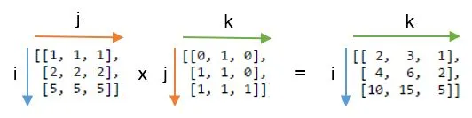
Ok Show Me an Example of Einsum

Let’s say we have two matrices A and B that we want to multiply them element-wise and then take sum for axis = 1 (row wise)

A = np.array([0, 1, 2]) # shape (3,)

B = np.array([[ 0,  1,  2,  3], # (3, 4)
              [ 4,  5,  6,  7],
              [ 8,  9, 10, 11]])

Using einsum notation,

>>> np.einsum('i,ij->i', A, B)
array([ 0, 22, 76])

Without einsum, this would look like -

Multiply them.

>>> A * B
Traceback (most recent call last):
  File "<stdin>", line 1, in <module>
ValueError: operands could not be broadcast together with shapes (3,) (3,4)

But alas, my silly self forgot to reshape. You require the matrices to have same dimensions in order for broadcasting. Convert A from (3,) → (3, 1) (essentially a column vector)

>>> A = A[:, np.newaxis]
>>> A
array([[0],
       [1],
       [2]])

Now you can perform

>>> (A * B).sum(axis = 1)
array([ 0, 22, 76])

#  A gets broadcasted from (3, 1) to (3, 3) before multiplication
# [0 0 0]
# [1 1 1]
# [2 2 2]

Reiterating, with einsum all you need did was np.einsum(‘i,ij->i’, A, B).

Let’s try to understand how it works.

But how Does it Work

np.einsum('string specifying indices and operation ', matrix1, matrix2 …)

The string looks like i, ij->i - input indices -> output indices

i, ij - input specification (the dimensions/axis of the matrices to which we do operations. The comma separates the indices of different matrices.

i → output specification (desired shape)

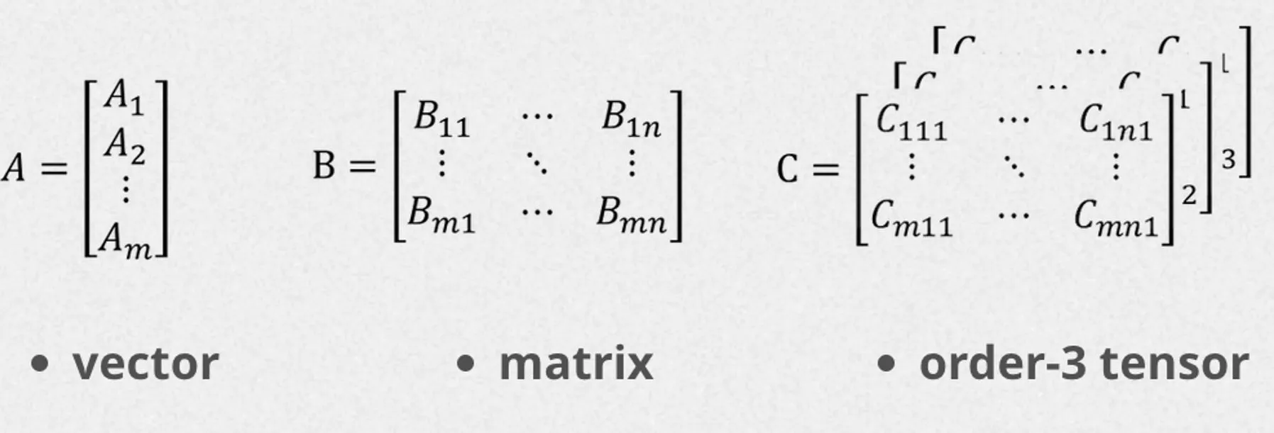
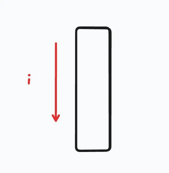
i corresponds to row of matrix A ij corresponds to row, column respectively for matrix B.

The specific letters that you can use in the string are arbitrary. You could have used something like a, ab->a. Just make sure that there is one label/index to represent each axis/dimension of the matrix.

Each letter/label e.g i, j represents the axis of the matrix/tensor that will be iterated over and can be expressed as a deeply nested set of for loops. There are a few important rules that you need to know after which it’s easy to understand einsum.

Some Rules

Note: I just write A[i][j] (pseudocode) as A[i, j] (numpy notation) for convenience

[1] Repeating letters between input arrays means that values along those axes will be multiplied together. The products make up the values for the output array.

i, ij->i

The result is going to be sum along axis = 1 for element wise product of A and B which means it’s going to be a row vector.

product[i] = A[i] * B[i][j]

If our einsum would have been something like bmhk, bhlm -> blhk then

product[b, l, h, k] = A[b, m, h, k] * B[b, h, l, m]

[2] Omitting a letter from the output means that values along that axis will be summed.

In simple words, any letter/index that doesn’t appear on the right hand side of the string is summed up over. We don’t put j on RHS since we want the sum along that dimension (column-wise)

output[i] += A[i] * B[i, j] # this is a tensor contraction

---

Tensor Contraction

Slight digression here. What we just did above is a tensor contraction.

It generalizes the concept of matrix multiplication to higher-dimensional arrays, or tensors. Summing over the product of paired indices between two tensors, resulting in a new tensor with reduced dimensionality. This is what einsum does.

Mathematically, the above operation can be expressed as

$$result[i]=∑jA[i]·B[i,j]$$

1. For each value of i, the elements of A[i] are multiplied with the corresponding elements of B[i,j] along the j axis.
2. The products are summed over the j axis, effectively reducing the dimensionality of the result.
3. The resulting tensor has shape [i], as specified by the output indices.

---

Below is how above einsum would look if we wrote it in the form of nested for loops (summations are for inner most for loops).

# for loop for above einsum
result = np.zeros(A.shape[0])
for i in range(A.shape[0]):
    for j in range(B.shape[1]):
        result[i] += A[i] * B[i, j]

But why is it faster? It didn’t require reshaping hence avoiding overhead of creating a temporary array A[:, np.newaxis] * B. It simply sums the products along the rows as it goes. That comples explanation for our first example.

[3] We can return the unsummed axes in any order we like.

This is sort of equivalent to reshaping/rearrange.

For example, transpose will be np.einsum('ij->ji', A)

>>> A = np.array([[1, 2, 3],
...               [4, 5, 6],
...               [7, 8, 9]])
>>>
>>> # Perform transpose using einsum
>>> A_transpose = np.einsum('ij->ji', A)
>>> A_transpose
array([[1, 4, 7],
       [2, 5, 8],
       [3, 6, 9]])

---

Sum of All Elements

np.einsum('ij->', A) - omitting both i, j means summation happens along these dimensions.

# Perform summation using for loop
sum_loop = 0
for i in range(A.shape[0]):
    for j in range(A.shape[1]):
        sum_loop += A[i, j] * 1

---

Trace

np.einsum(’ii->’, A) For trace of matrix (sum of diagonal elements)

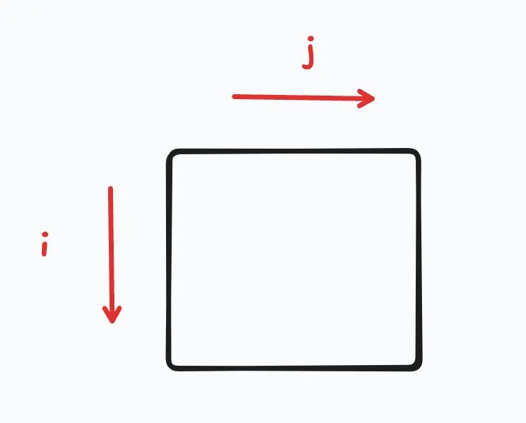
Matrix Multiplication in Einsum

$$Cij=∑kAikBkj$$

A better example to demonstrate einsum is matrix multiplication. Above can be expressed in for three nested for loops (brute force matrix multiplication algorithm). Here’s an animation.

k is repeated which means product happens along it. k is not in the output specification summation. k is called summation index.

All indices in einsum format string can be partitioned in two sets: free indices and summation indices

• Free indices  are the indices used in the output specification (right hand side of string). They are associated with the  outer for loops.
• Summation indices  are all other indices: those that appear in the argument specifications but  not  in the output specification. They are so called because they are  summed out  when computing the output tensor. They are associated with the inner for loops.

You could also mention matrix multiplication as np.einsum(’ij,jk→ik’, A, B) and it would be still valid (as I mentioned earlier that the letters are arbitrary).

Matrix Product Tranpose

Let’s say you want to get transpose of matrix product i.e (A @ B).T

np.einsum('ij,jk->ki', A, B) Note how we just rearranged ik to ki and that’s a transpose.

Observations for Nested Loops

ij, jk->ik - the number of unique indices in the string = number of nested loops

The order of nested loops will follow the order of the right hand side/output specification of the string.

index not present on right side - summation index, always present in the innermost loop

---

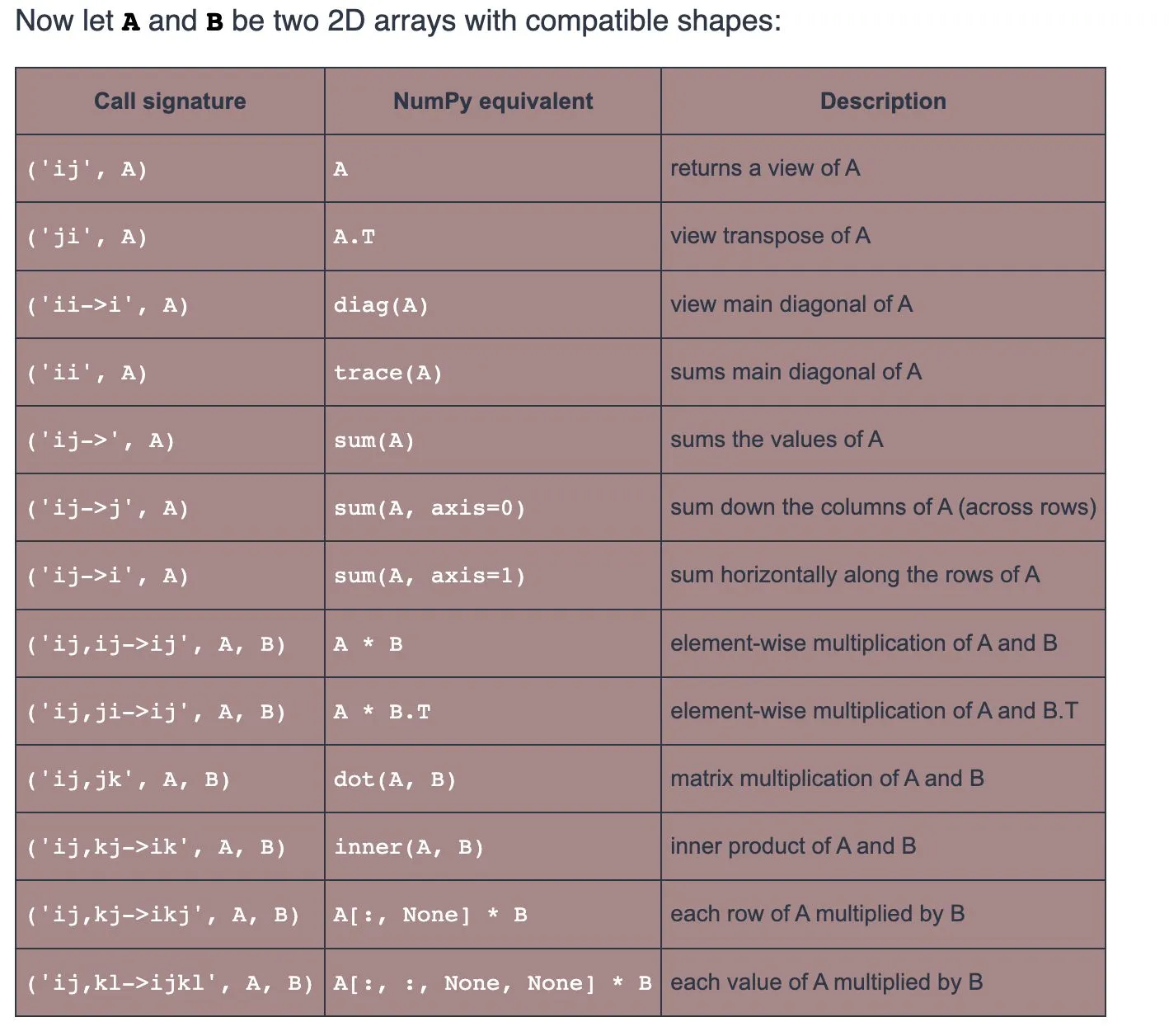
Here’s a list of operations to practice mentally (image stolen from post 4)

Ok, that’s a lot to digest. Take a break fellow shape rotator for in the next section, we shall dive deep into a simple Jax transformer implementation and witness einsum in action on the frontlines of deep learning.

Part 2 Decoding Simple Jax Transformer

Shoutout again to Mr. xjdr for open source contribution of the jax transformer code.

It’s cleanly written and tested by him. He also clarified some of my doubts.

About Jax

Jax is somewhere middle in between of Numpy and Pytorch. Researchers mainly use Pytorch for research but for production loads, people are moving to Jax for being faster. You will see that it’s syntax is similar to numpy (but there is a huge emphasis on functional programming concepts like pure functions, immutable arrays etc.). It uses JIT (just in time compilation to fasten things up.

Next we try to decode this simple transformer implementation in Jax.

---

Simple Jax Transformer

According to Mr. _xjdr, “this is a decoder only, from the early noam era pre RoPE transformer”

from typing import List, NamedTuple

import jax
import jax.numpy as jnp

class LayerWeights(NamedTuple):
  attn_norm: jax.Array
  ffn_norm: jax.Array
  w_q_dhk: jax.Array
  w_k_dhk: jax.Array
  w_v_dhk: jax.Array
  w_o_hkd: jax.Array
  w1: jax.Array
  w2: jax.Array
  w3: jax.Array

class XfmrWeights(NamedTuple):
  tok_embeddings: jax.Array
  layer_weights: List[LayerWeights]
  norm: jax.Array
  output: jax.Array

def norm(x, w, eps: float = 1e-6):
    return w * (x * jax.lax.rsqrt(jax.lax.pow(x, 2).mean(-1, keepdims=True) + eps))

def attention(input_bld, params):
    """
    B: batch size
    L: sequence length
    M: memory length
    D: model dimension
    H: number of attention heads in a layer
    K: size of each attention key or value
    """
    normalized_bld = norm(input_bld, params.attn_norm)
    query_blhk = jnp.einsum('bld,dhk->blhk', normalized_bld, params.w_q_dhk)
    key_blhk = jnp.einsum('bld,dhk->blhk', normalized_bld, params.w_k_dhk)
    value_blhk = jnp.einsum('bld,dhk->blhk', normalized_bld, params.w_v_dhk)
    logits_bhlm = jnp.einsum('blhk,bmhk->bhlm', query_blhk, key_blhk)
    _, l, h, k = query_blhk.shape
    logits_bhlm = logits_bhlm / jnp.sqrt(k)
    mask = jnp.triu(jnp.ones((l, l)), k=1).astype(input_bld.dtype)
    logits_bhlm = logits_bhlm - jnp.inf * mask[None, None, :, :]
    weights_bhlm = jax.nn.softmax(logits_bhlm, axis=-1)
    wtd_values_blhk = jnp.einsum('blhk,bhlm->blhk', value_blhk, weights_bhlm)
    out_bld = jnp.einsum('blhk,hkd->bld', wtd_values_blhk, params.w_o_hkd)
    return out_bld

def ffn(x: jax.Array, w1: jax.Array, w2: jax.Array, w3: jax.Array) -> jax.Array:
  return jnp.dot(jax.nn.silu(jnp.dot(x, w1)) * jnp.dot(x, w3), w2)

def transformer(tokens: jax.Array, params: jax.Array) -> jax.Array:
  x = params.tok_embeddings[tokens]
  def scan_fn(h, layer_weights):
    h += attention(h, layer_weights)
    h += ffn(norm(h, layer_weights.ffn_norm), layer_weights.w1, layer_weights.w2, layer_weights.w3)
    return h, None
  h, _ = jax.lax.scan(scan_fn, x, params.layer_weights)
  h = norm(h, params.norm)
  logits = jnp.dot(h, params.output.T)
  return logits

if __name__ == '__main__':
  vocab_size = 32000
  dim = 4096
  hidden_dim = 14336
  n_layers = 1
  n_heads = 32
  head_dim = dim // n_heads

  layer_weights = LayerWeights(
      attn_norm=jnp.ones((n_layers, dim,)),
      ffn_norm=jnp.ones((n_layers, dim,)),
      w_q_dhk=jnp.zeros((n_layers, dim, n_heads, head_dim)),
      w_k_dhk=jnp.zeros((n_layers, dim, n_heads, head_dim)),
      w_v_dhk=jnp.zeros((n_layers, dim, n_heads, head_dim)),
      w_o_hkd=jnp.zeros((n_layers, n_heads, head_dim, dim)),
      w1=jnp.zeros((n_layers, dim, hidden_dim)),
      w2=jnp.zeros((n_layers, hidden_dim, dim)),
      w3=jnp.zeros((n_layers, dim, hidden_dim))
    )
  params = XfmrWeights(tok_embeddings=jnp.ones((vocab_size, dim)), layer_weights=layer_weights, norm=jnp.ones((dim,)), output=jnp.ones((vocab_size, dim)))
  tokens = jnp.array([123,234,234,345,446](123,234,234,345,446))
  out = transformer(tokens, params)
  print(f'{out.shape=}')

Let’s first look at the simplest one —> FFN Then we proceed to top down with transformer block and finally into the multi-head attention block (lots of einsum but nothing to be afraid of)

---

Feed forward Network / Mlp

def ffn(x: jax.Array, w1: jax.Array, w2: jax.Array, w3: jax.Array) -> jax.Array:
  return jnp.dot(jax.nn.silu(jnp.dot(x, w1)) * jnp.dot(x, w3), w2)

$$FFN(x,W1,W2,W3)=(SiLU(xW1)⊙(xW3))W2$$

Transformer layer have the feedforward network typically after the attention blocks to increase non-linearity and capture the information learnt by the attention heads. This MLP has two layers of linear transformation with a SiLU activation.

1. Two parallel linear transformations: dot(x, W1) and dot(x, W3)
2. SiLU activation applied to dot(x, W1)
3. Element-wise multiplication of the result from step 2 with dot(x, W3)
4. Final linear transformation: dot product of the result from step 3 with W2

---

Transformer Block

Before we go to the transformer block, I want to talk about jax.lax.scan function.

When you have a for loop where you update a value in each step and want to return the final result along with all the intermediate values from each step (np.stack), you use jax.lax.scan. Under the hood, it can unroll loops (and do some jit stuff) for speedup. Another purpose is to express the scan_fn as a pure function (avoid mutable states).

from jax import lax

def cumulative_sum(accumulated_sum, current_element):
    """
    - \`accumulated_sum\`: The accumulated sum from the previous loop iteration.
    - \`current_element\`: The current array element being processed.
    """
    new_sum = accumulated_sum + current_element
    return new_sum, new_sum  # ("carryover", "accumulated")

initial_sum = 0
final_sum, cumulative_sums = lax.scan(cumulative_sum, initial_sum, array)

In a transformer, we need to apply the same operations (attention and feed-forward) multiple times, once for each layer. This is where jax.lax.scan comes in handy.

Instead of writing a loop to apply these operations, we can use scan to do it more efficiently. We use it to write the (Multi-head attention + FFN) block repeatedly.

The transformer function shown is a decoder-decoder only implementation (causal masking is the hint). There is no positional encoding.

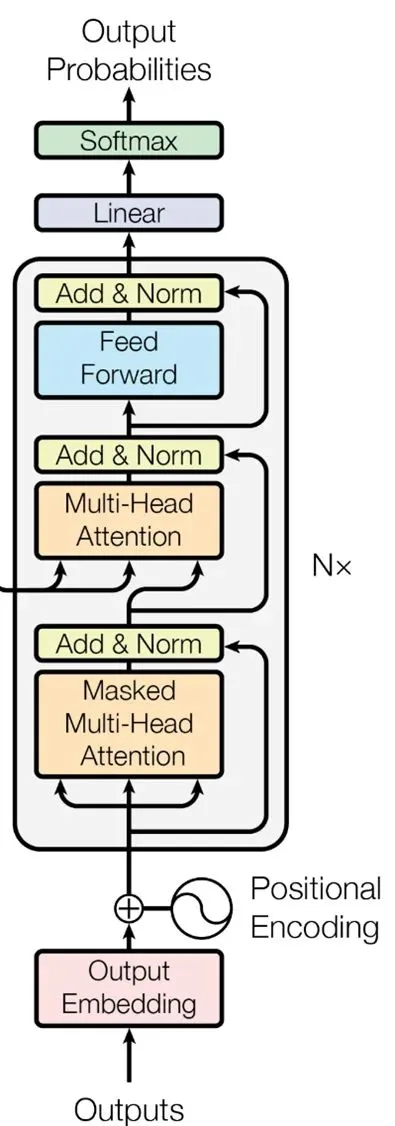
def transformer(tokens: jax.Array, params: jax.Array) -> jax.Array:
  x = params.tok_embeddings[tokens]
  def scan_fn(h, layer_weights):
    h += attention(h, layer_weights)
    h += ffn(norm(h, layer_weights.ffn_norm), layer_weights.w1, layer_weights.w2, layer_weights.w3)
    return h, None
  h, _ = jax.lax.scan(scan_fn, x, params.layer_weights)
  h = norm(h, params.norm)
  logits = jnp.dot(h, params.output.T)
  return logits

h += attention(h, layer_weights)
h += ffn(norm(h, layer_weights.ffn_norm), layer_weights.w1, layer_weights.w2, layer_weights.w3)

These are the residual connections as you can see in the diagram too. We are collecting output from each hidden layer

---

Next section, we look into the attention block after all “Attention is all you need”

Attention Block

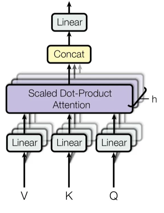
Attention is at the heart of transformers, allowing the model to discern which parts of the input to attend to. In this section, we look at the multi-head attention block implementation.

---

Single-Head Attention: In single-head attention h = 1

Before jumping to full attention implementation, let’s just take a minute to go through common einsums here.To understand the einsum involved for creating query matrix. We are projecting the input into a single attention space.

query_blk = jnp.einsum('bld, dk -> blk', normalized_bld, params.w_q_dk)

Here, ‘b’ is batch size, ‘l’ is sequence length, ‘d’ is the model dimension, and ‘k’ is the query/key dimension (latent key space). normalized_bld is the input, params.w_q_dk are learnable weights.

Note: elements in q refers to the token for which attention is calculated, elements in k (latent space) are about tokens that can be attended to

The above einsum is basically a matrix multiplication / dot product between each token’s embedding and set of learnt weight vectors. ld, dk -> lk

More formally, this projection transforms each token’s representation from ‘d’ dimensions to ‘k’ dimensions. Here, the h i.e number of heads i 1.

---

Multi-head attention: However, we are using Multi-Head attention in our implementation. You can think of it as single head attention repeated h times.

Honestly I was not 100% clear on why we do summation upon d. Mr. xjdr says think of it as “for each of these token embeddings, tell me everything you know about them, per attention head, in the latent space of size dim”

If single-head is about looking at a scene through a single lens, multi-head is looking at same scene with multiple lenses, each having different perspective.

query_blhk = jnp.einsum('bld, dhk -> blhk', normalized_bld, params.w_q_dhk)

Notice that this is just matrix multiplication again with an extra dimension (h) where the summation is taking across the d axis. Now we are projecting the input into h attention subspaces.

---

Now let’s see the full multi-head attention block.

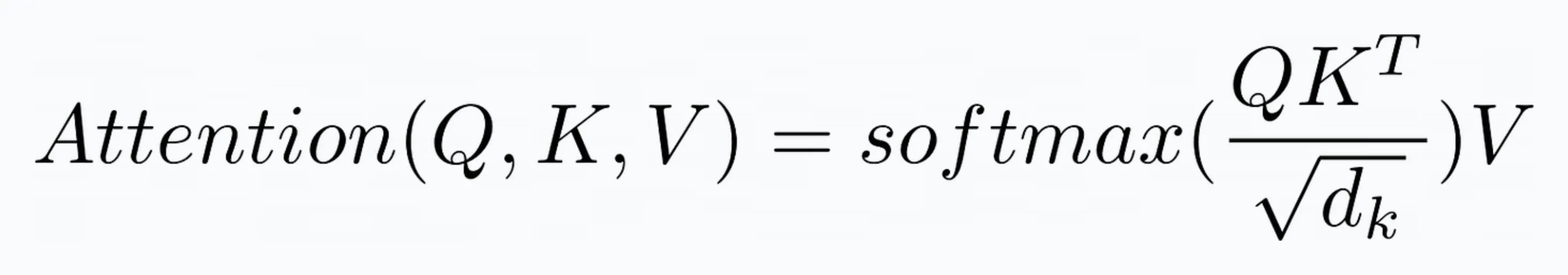
Below is the scaled dot product attention equation. This is calculated for h heads (hence mutli-head)

def attention(input_bld, params):
    """
    Implements multi-head self-attention mechanism.

    B: batch size
    L: sequence length
    M: memory length (same as L for self-attention)
    D: model dimension
    H: number of attention heads in a layer
    K: size of each attention key or value
    """

    # Layer normalization
    normalized_bld = norm(input_bld, params.attn_norm)

    # Linear projections to obtain query, key, and value
    # Notice they are just matrix multiplications with an extra batch dim
    # XWq operation
    query_blhk = jnp.einsum('bld,dhk->blhk', normalized_bld, params.w_q_dhk)
    # XWk operation
    key_blhk = jnp.einsum('bld,dhk->blhk', normalized_bld, params.w_k_dhk)
    # XWv operation
    value_blhk = jnp.einsum('bld,dhk->blhk', normalized_bld, params.w_v_dhk)

    # Compute attention scores (dot product of queries and keys)
    # Notice that keys don't have sequence length, they have memory length
    # Memory is the length of context model can attend to
    # i.e how many previous tokens it can refer to
    logits_bhlm = jnp.einsum('blhk,bmhk->bhlm', query_blhk, key_blhk)


    # Get shape for scaling
    _, l, h, k = query_blhk.shape

    # Scale dot products by sqrt(d_k)
    logits_bhlm = logits_bhlm / jnp.sqrt(k)


    # Create causal mask to prevent attending future tokens
    # causal mask (lower triangular)
    mask = jnp.triu(jnp.ones((l, l)), k=1).astype(input_bld.dtype)

    # Apply mask (set upper triangular region to -inf)
    logits_bhlm = logits_bhlm - jnp.inf * mask[None, None, :, :]

    # Apply softmax to get attention weights
    weights_bhlm = jax.nn.softmax(logits_bhlm, axis=-1)

    # Compute weighted sum of values
    wtd_values_blhk = jnp.einsum('blhk,bhlm->blhk', value_blhk, weights_bhlm)

    # Final linear projection
    out_bld = jnp.einsum('blhk,hkd->bld', wtd_values_blhk, params.w_o_hkd)

    return out_bld

Why summation upon k in logits_bhlm = jnp.einsum('blhk,bmhk->bhlm', query_blhk, key_blhk)? Since k contains information about which token embeddings to attend to in each head, that’s why we collect information across that axis.

I hope you have a better understanding of einsum and know a bit more about transformers and jax more than before. Please upvote and share if you liked.

I am also looking for GenAI(LLMs) oriented roles, at big companies or funded startups (India (hybrid) and US/EU remote roles). Open for contract roles too. If you are looking out, please drop a DM On twitter or send me a “Hi” on hgirl3078@gmail.com.

My background is ~2 years of production experience at backend/generalist software engineering at a mid sized USA based fintech company. I have also dabbled into deep learning(college era) and applied LLMs(recently).

A recent project you may find interesting - codeQA. A chat-with-a-codebase project utilizing tree-sitter to generate AST trees and construct a codebase index for embeddings. Then I implement a simple top-K RAG pipeline with meta-characteristic search, HyDE, LanceDB, BM-25 etc. to get the chatting working.

• Part 1: Learnings from codeQA - Tree-sitter
• Part 2: Learnings from codeQA - Improving Retrieval